The most popular tool for detecting chaos in experimental data is calculation of the correlation dimension using the method of Grassberger and Procaccia (Phys. Rev. Lett. 50, 346-349 (1983)). The idea is to construct a function C(r) proportional to the probability that two arbitrary points on the orbit in state space are closer together than r. This is usually done by calculating the separation between every pair of N data points and sorting them into bins of width dr proportional to r. The correlation dimension is given by D2 = d log(C) / d log(r) in the limit dr --> 0, r --> 0, and N --> infinity. These limits are inherently incompatible for a finite data set, and for many attractors, the computed value of D2 converges very slowly. In the original Grassberger-Procaccia paper, data (with N = 15,000) are shown only for the Henon map and Lorenz model, and it turns out that these cases are exceptional in their rapid convergence. For this reason, the literature is devoid of credible calculations of the correlation dimension for most model chaotic systems, including the logistic map, the Rossler attractor, and the Chirikov map.
To study convergence of standard chaotic systems it is necessary to generate large data sets, possibly exceeding the memory of the computer. Since new data can be generated inexpensively compared to the computational cost of performing the correlation calculation, a good strategy is to save the data in a circular buffer. Each new iterate replaces the oldest point in the buffer, which is then discarded. As each new point is added to the buffer, its separation from each of the previous points is calculated and sorted into bins. A few of the most recent points are excluded to avoid errors due to temporal correlation. The number of such points is small and can be estimated from the Lyapunov exponent. For example, with the Henon map, the largest Lyapunov exponent is known to be about 0.603 bits/iteration, and so after 133 iterations in 80-bit precision, no temporal correlations should remain. For the work reported here, a buffer of 32767 points was used, and the most recent 767 points were ignored.
The accuracy with which the correlation dimension can be calculated is dictated by the total number of pairs of data points that are correlated. With abundant data, there is thus a premium on calculating and binning the separations as quickly as possible. The Euclidean separation between two points (x1, y1) and (x2, y2) is calculated from r = [(x2 - x1)2 + (y2 - y1)2]1/2. It has been proposed to use other measures such as the absolute norm, r = |x2 - x1| + |y2 - y1|, or the maximum norm, r = max[|x2 - x1|, |y2 - y1|], but these methods tend to give inferior results. Note, however, that it is not necessary to perform the square root; it is just as good to bin the values of r2 as it is to bin the values of r, since log(r2) = 2 log(r).
With bins of width dr proportional to r, there are several strategies for sorting the separations into the appropriate bin. The conceptually simplest method is to generate a bin index by taking the integer part of log(r2). Calculation of the logarithm typically limits the speed of this method. A clever scheme is to make use of the fact that computers store floating point numbers with a mantissa and an integer exponent of 2. Thus it is possible to find the integer part of log2(r2) by extracting the appropriate bits of the variable r2. This method automatically gives 2 / log10(2) = 6.64 bins per decade, which is reasonable and sufficient for our purposes.
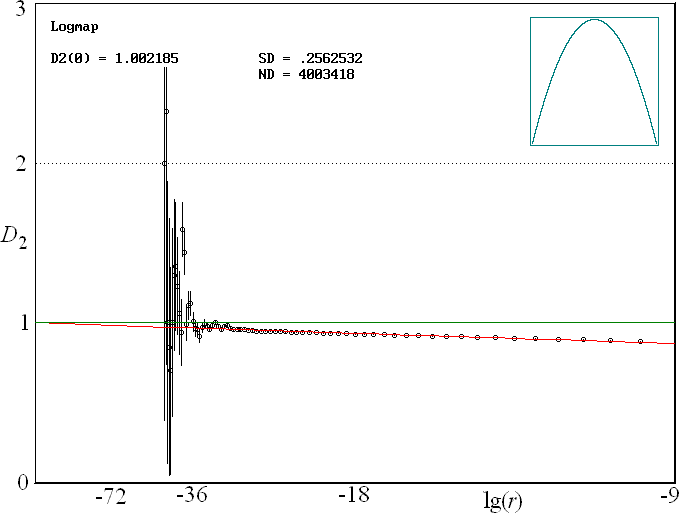
As a numerical example, consider the logistic map xn+1 = 4xn(1-xn), for which the correlation dimension is known to be exactly 1.0. This is a case for which D2 converges very slowly as r --> 0. In fact, it can be shown that D2 = 1 + 1/loge(r) in the limit of small r. Thus to get a result accurate to 1%, requires r = 3.72 x 10-44. To have even one pair of points with a separation that small would require the order of 1022 data points. Furthermore, calculation of such a small r would underflow the precision of the computer floating point numbers. However, if the functional form of D2(r) is known, it is possible to collect data for some convenient range of r and then extrapolate to the limit r = 0. For the logistic map, a plot of D2 versus 1/log2(r) is shown below:

Even with over 4 million fully correlated data points, the value of D2 is still significantly below 1.0, but extrapolation of the least squares fit (the red line) to r = 0 gives a value of D2(0) = 1.002185. In the plot above, the error bars are calculated assuming the statistical error for the number of points in each bin is equal to the square root of that number and that the fluctuations in the number in adjacent bins is uncorrelated. These assumptions are probably optimistic.
The reason for the slow convergence is the highly non-uniform measure on the unit interval. For the logistic map, the probability distribution is given by P(x) = 1/pi[x(1-x)]1/2. The infinite value of P at x = 0 and x = 1 is a result of the parabolic nature of the map and the fact that a finite interval of x values near x = 0.5 map into the same point. Thus we would expect this kind of dependence for any unimodal 1-D map with a quadratic maximum. Presumably this dependence is universal for a wide class of maps.
More generally we define p = log(C) and q
= log(r)
and suppose that p(q) is of the form p
= A
+ D2(0)q + f(q), where f(q)
is a function whose derivative df/dq approaches
zero as r
--> 0. For the logistic equation, f(q) = loge(-q).
Assuming
this functional form is generic with f(q) = B
loge(-q), a least squares fit to various
dynamical
systems gives the following results:
|
|
|
|
|
| Logistic map (A = 4) | 4.2 x 10⁶ | 0.92 | 1.01 |
| Logistic map (A = 3.9) | 1.1 x 10⁶ | 0.68 | 0.99 |
| Logistic map (A = 3.6) | 1.3 x 10⁶ | 0.53 | 0.98 |
| Sine map | 1.1 x 10⁶ | 0.83 | 1.00 |
| 2 logistic maps (A = 4) | 1.9 x 10⁶ | 1.35 | 1.97 |
| 3 logistic maps (A = 4) | 1.1 x 10⁶ | 1.81 | 2.92 |
| Uniform random data | 9.0 x 10⁵ | 0.27 | 1.03 |
| 2-D uniform random data | 1.1 x 10⁶ | 0.30 | 2.04 |
| Alpha = 0.5 map | 1.7 x 10⁶ | 0.48 | 1.06 |
| Alpha = 1.5 map | 1.2 x 10⁶ | 0.37 | 1.03 |
| Alpha = 3 map | 1.7 x 10⁶ | 2.04 | 0.82 |
| Henon map (b = 0.3) | 3.3 x 10⁶ | 0.13 | 1.22 |
| Henon map (b = 0.1) | 1.1 x 10⁶ | 0.58 | 1.13 |
| Lozi map | 1.4 x 10⁶ | 0.05 | 1.40 |
| Chirikov map (k = 1) | 1.2 x 10⁶ | -0.16 | 1.89 |
| Arnold cat map | 1.1 x 10⁶ | -0.04 | 1.99 |
| Lorenz attractor | 2.3 x 10⁶ | -0.27 | 2.02 |
| Rossler attractor | 3.0 x 10⁶ | 0.94 | 2.01 |
| Ueda attractor | 2.1 x 10⁶ | 0.50 | 2.68 |
| Simplest quadratic | 2.2 x 10⁶ | 1.71 | 2.12 |
| Simplest piecewise linear | 2.1 x 10⁶ | 2.95 | 2.25 |
References:
J. C. Sprott,
and G.
Rowlands, Improved
Correlation Dimension Calculation, International
Journal of Bifurcation and Chaos 11, 1865-1880 (2001).
J. C. Sprott,
Chaos and Time-Series Analysis
(Oxford University Press, 2003), pp.329-336.